Day 2: Simulate Data

Sara Tyo, Department of Statistics, University of California, Irvine

2024-07-09

What is Data Simulation?

  • Definition: Data simulation is the process of generating synthetic data that mimics real-world data characteristics.

  • Purposes:

    • Exploration: Understand data distributions and relationships.

    • Analysis: Test hypotheses, evaluate models, and simulate scenarios.

    • Training: Prepare datasets for training machine learning models.

Example

Code
# Generating example data
set.seed(321)
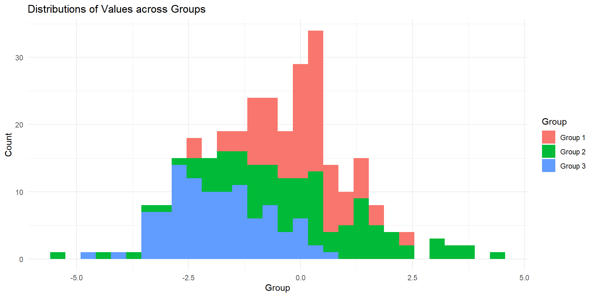
data1 <- rnorm(100, mean = 0, sd = 1)   # Distribution 1: Mean 0, SD 1
data2 <- rnorm(100, mean = 0, sd = 2)   # Distribution 2: Mean 0, SD 2
data3 <- rnorm(100, mean = -2, sd = 1)  # Distribution 3: Mean -2, SD 1

# Creating a data frame for plotting
df <- data.frame(
  Group = rep(c("Group 1", "Group 2", "Group 3"), each = 100),
  Value = c(data1, data2, data3)
)

Explanation:

set.seed()

1. Purpose:

  • Reproducibility: When you generate random numbers in R using functions like rnorm() (for normal distribution), runif() (for uniform distribution), etc., the numbers are pseudo-random. This means they appear random but are actually generated using a deterministic algorithm that starts from a specific initial state (seed).

  • rnorm: Function in R to generate random numbers from a normal distribution.

  • Parameters:

    • mean: Mean of the distribution.

    • sd: Standard deviation of the distribution.

  • Generates three sets (data1, data2, data3) of 100 random numbers each with different means and standard deviations.

Histograms

  • Show histograms of data1, data2, and data3.

  • Discuss the impact of mean and standard deviation on the shape and spread of the distributions.

Code
library(ggplot2)
ggplot(df, aes(x = Value, fill = Group, stat="count")) +  
  geom_histogram() +  
  labs(title = "Distributions of Values across Groups",
       x = "Group", y = "Count") +
  theme_minimal()

Importance of Simulation in Data Analysis

  • Advantages:

    • Flexibility: Easily generate data to fit specific scenarios.

    • Control: Adjust parameters to simulate various conditions.

    • Testing: Validate statistical methods and models.

  • Applications:

    • Financial modeling, risk assessment, predictive analytics, etc.

Practical Applications

  • Example: Simulating customer purchase behavior in an online store.

    • Variables: Purchase frequency, average order value, time between purchases.

    • Purpose: Predict sales, optimize marketing strategies.

  • Possible way of simulating

    Code
    library(ggplot2)
    library(dplyr)
    
    # Set seed for reproducibility
    set.seed(123)
    
    # Number of customers
    num_customers <- 1000
    
    # Simulate purchase frequency
    purchase_frequency <- round(runif(num_customers, min = 1, max = 20))
    # Simulate average order value
    average_order_value <- rnorm(num_customers, mean = 50, sd = 10)
    # Simulate time between purchases (in days)
    time_between_purchases <- round(rnorm(num_customers, mean = 30, sd = 10))
    
    # Create a data frame
    customer_data <- data.frame(
      customer_id = seq(1, num_customers),
      purchase_frequency = purchase_frequency,
      average_order_value = average_order_value,
      time_between_purchases = time_between_purchases
    )

Conclusion

  • Summary:

    • Data Simulation as a Powerful Analytical Tool Data simulation stands as a cornerstone in modern data science, providing robust capabilities for understanding and analyzing complex datasets.

    • By generating synthetic data that mirrors real-world scenarios, businesses and researchers alike can uncover hidden patterns, test hypotheses, and make informed decisions.