Day 2: Introduction to Estimation

Zhaoxia Yu, Department of Statistics, University of California, Irvine

2024-07-14

Introduction

For a population, two important parameters are population mean and population variance, denoted as \(\mu\) and \(\sigma^{2}\) respectively, of a random variable.
Parameters are unknown in general.
We shall use observed data to estimate the unknown parameters.
In this process, we often provide
- a point estimate
- uncertainty, such as standard error of the point estimate or a confidence interval

Let \(X_{1}, X_{2}, \ldots, X_{n}\) denote a random sample of size \(n\) from a population with population mean \(\mu\) and population variance \(\sigma^2\).
The sample mean: \[ \begin{equation*} \bar{X} = \frac{\sum_{i=1}^{n}X_{i}}{n}=\frac{X_1+\cdots+X_n}{n}. \end{equation*} \]
The sample variance

\[ S^2= \frac{\sum_{i=1}^{n}(X_{i}-\bar X)^2}{n-1}=\frac{(X_1-\bar X)^2+\cdots+(X_n-\bar X)^2}{n-1}. \]

The sample mean \(\bar{X}\) can be used as an estimator for \(\mu\). Notation: \[\hat\mu=\bar X\]
The estimator itself is considered as a random variable since it value can change.
Similarly, the sample variance \(S^2\) can be used to estimate \(\sigma^2\). Notation: \(\hat\sigma^2=S^2\).

Using a sample \(x_{1}, x_{2}, \ldots, x_{n}\), we can compute

\[ \begin{equation*} \bar{x} = \frac{\sum_{i=1}^{n}x_{i}}{n} \end{equation*} \]

\[ \begin{equation*} s^{2} = \frac{\sum_{i=1}^{n}(x_{i} - \bar{x})^{2}}{n-1}. \end{equation*} \]

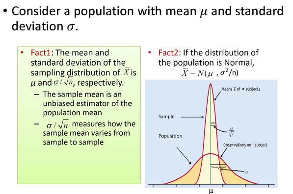
As shown in the previous slide, if the true distribution is \(N(\mu, \sigma^2)\), then \[\bar X \sim N(\mu, \frac{\sigma^2}{n}) \mbox{ and } \frac{\bar X-\mu}{\sigma/\sqrt{n}} \sim N(0, 1)\]
If the sample is not from a normal distribution, in many cases, as long as the sample size \(n\) is large enough, the normal distribution still works well.
The underlying theories related are
- the central limit theorem
- law of large numbers

Confidence intervals based on Z-critical values have the form of \(\bar x \pm Z_{crit} \frac{\sigma}{\sqrt{n}}\). In practice, we don’t konw \(\sigma\), so we use

\[\bar x \pm Z_{crit} \frac{s}{\sqrt{n}}.\]

Use the 68-95-99.7 rule
- a 95% confidence interval (CI) is \(\bar x \pm 2 \frac{s}{\sqrt n}\).
- a 99.8% confidence interval (CI) is \(\bar x \pm 3 \frac{s}{\sqrt n}\).

\[\frac{\bar X-\mu}{s/\sqrt{n}} \sim t_{n-1}\]

\[\bar x \pm t_{crit} \frac{s}{\sqrt{n}},\] where \(t_{crit}\) depends on both the sample size \(n\) and the chosen confidence level.

We refer to \(s/\sqrt{n}\) as the standard error of the sample mean \(\bar{X}\).
We can write the confidence interval as \[\begin{equation*} \bar{x} \pm t_{\mathrm{crit}}\times SE \end{equation*}\]
The term \(t_{\mathrm{crit}}\times SE\) is called the margin of error for the given confidence level.
It is common to present interval estimates for a given confidence level as \[\begin{equation*} \textrm{Point estimate} \pm\textrm{Margin of error.} \end{equation*}\]
Note, in many articles, people also present mean \(\pm\) SD.

Estimate the volume of hippocampus for women between 40 and 50 years old

Code

alzheimer_data <- read.csv('data/alzheimer_data.csv')
dim(alzheimer_data)

[1] 2700   57

Code

alzheimer_subset =alzheimer_data[alzheimer_data$age<=50 & alzheimer_data$age>40 & alzheimer_data$female==1, ]
dim(alzheimer_subset)

[1] 70 57

Code

hippo=alzheimer_subset$lhippo + alzheimer_subset$rhippo
#estimate of mean
mean(hippo)

[1] 6.470666

Code

#standard error
sd(hippo)/sqrt(length(hippo))

[1] 0.1023539

Code

#a 95% c.i. using z-critical value
mean(hippo) - 2*sd(hippo)/sqrt(length(hippo))

[1] 6.265958

Code

mean(hippo) + 2*sd(hippo)/sqrt(length(hippo))

[1] 6.675374

Code

mean(hippo) - qnorm(0.975)*sd(hippo)/sqrt(length(hippo))

[1] 6.270056

Code

mean(hippo) + qnorm(0.975)*sd(hippo)/sqrt(length(hippo))

[1] 6.671276

Code

mean(hippo) - qt(0.975, df=length(hippo)-1)*sd(hippo)/sqrt(length(hippo))

[1] 6.266475

Code

mean(hippo) + qt(0.975, df=length(hippo)-1)*sd(hippo)/sqrt(length(hippo))

[1] 6.674856