Multivariate Analysis Lecture 14: More on Classification
2025-05-14
Introduction
Outline
- Review of LDA
- QDA
- Decision theory
- Equal costs
- Unequal costs
Review of LDA
Linear Discrminant Analysis
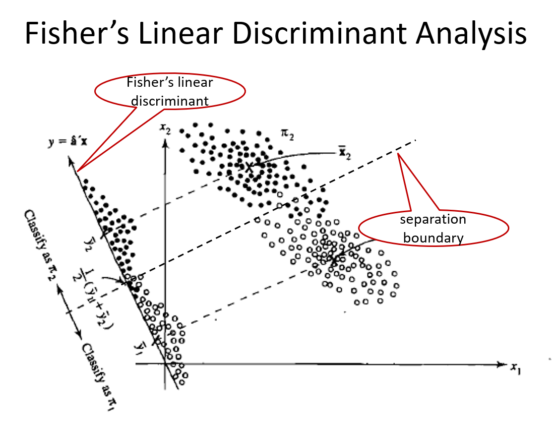
FLDA: Maximum Separability for Two-Class Problems
The maximization problem is \[\operatorname*{argmax}_a \frac{a^T(\bar {\mathbf X}_1 - \bar {\mathbf X}_2)(\bar {\mathbf X}_1 - \bar {\mathbf X}_2)^Ta}{a^T \boldsymbol \Sigma a}\]
Use an argument similar to PCA, such \(a\) is the first eigenvector of \(\boldsymbol \Sigma ^{-1}(\bar {\mathbf X}_1 - \bar {\mathbf X}_2)(\bar {\mathbf X}_1 - \bar {\mathbf X}_2)^T\).
We can show that \(a=\mathbf S_p^{-1}(\bar {\mathbf X}_1 - \bar {\mathbf X}_2)\).
The linear function \[f(x)=a^T x \mbox{ where } a=\mathbf S_p^{-1}(\bar {\mathbf X}_1 - \bar {\mathbf X}_2)\] is called Fisher’s linear discriminant function.
Allocate New Observations
Consider an observation \(X_0\). We compute \[f(X_0)=a^T X_0\] where \(a=\mathbf S_p^{-1}(\bar {\mathbf X}_1 - \bar {\mathbf X}_2)\)
Let \[m=a^T \frac{\bar {\mathbf X}_1 + \bar {\mathbf X}_2}{2}=\boldsymbol (\bar {\mathbf X}_1 - \bar {\mathbf X}_2)^T \mathbf S_p^{-1}\frac{\bar {\mathbf X}_1 + \bar {\mathbf X}_2}{2}\]
Allocate \(X_0\) to
- class 1 if \(f(X_0)>m\)
- class 2 if \(f(x_0)<m\)
g-Class Problems
- Measure separation using F statistic \[\begin{aligned} F(a) &= \frac{MSB}{MSW}=\frac{SSB/(g-1)}{SSW/(n-g)}\\ &= \frac{\sum_{i=1}^g n_i (\bar Y_{i.}^{(1)} -\bar Y_{..}^{(1)})^2/(g-1)}{\sum_{i=1}^g (n_i-1)S_{Y_i^{(1)}}^2/(n-g)}\\ &=\frac{a^T \sum n_i (\bar X_{i.} -\bar X_{..})(\bar X_{i.}-\bar X_{..})^T a}{a^T \sum_{i=1}^g\sum_{j=1}^{n_i} (X_{ij} -\bar X_{i.})(X_{ij}-\bar X_{i.})^T a}\frac{n-g}{g-1}\\ &= \frac{a^T \mathbf B a}{a^T \mathbf W a}\frac{n-g}{g-1} \end{aligned}\] where \(n=\sum_{i=1}^g n_i\), \(\mathbf B\) is the between-group sample covariance matrix, and \(\mathbf W\) is the within-group sample covariance matrix.
Linear Discriminants
The first linear discriminant is the linear function that maximizes \(F(a)\). It can also be shown that the first linear discriminant is given by the first eigenvector of \(\mathbf W ^{-1} \mathbf B\), i.e., \[Y_{ij}^{(1)}=\gamma_1^T X_{ij}\] where \(\gamma_1\) is the first eigenvector of \(\mathbf W ^{-1} \mathbf B\).
Similarly, for \(k=1, \cdots, rank(\mathbf B)\), the \(k\)th linear discriminant is given by the \(k\)th eigenvector of \(\mathbf W ^{-1} \mathbf B\)
\[Y_{ij}^{(k)}=\gamma_k^T X_{ij}\]
Use the Linear Discriminants
Let \(X_0\) be a new observation. We allocate it to the group with the minimum distance defined by the Euclidean distance in space spanned by the linear discriminants.
Calculate \(Y_0^{(k)}=\gamma_k^T X_0\), the projection of \(X_0\) to the \(k\)th linear discriminant for \(k=1, \cdots, rank(B)\).
Calculate the distance between \((Y_0^{(1)}, \cdots, Y_0^{(rank(B))})\) and \((\bar Y_{i.}^{(1)}, \cdots, \bar Y_{i.}^{(rank(B))})\)
\[D^2(X_0, i) = \sum_{k=1}^{rank(B)} [Y_0^{(k)} - \bar Y_{i.}^{(k)}]^2\]
- Allocate \(X_0\) to \(\operatorname*{argmin}_i D^2(X_0, i)\).
Quadratic DA (QDA)
QDA for Two-Class Problems
- The LDA can be derived using likelihood functions under the assumptions
- Multivariate normal
- Equal covariance matrix
- The assumption of equal covariance matrix is not always a good approximation to the true covariance matrices
- If we relax this assumption, we will have QDA
QDA for Two-Class Problems
Let’s consider a two-class classification problem with \(n_1\) and \(n_2\) observations in classes 1 and 2, respectively.
Suppose we have two independent random samples
- Sample 1: \(X_{1j}\overset{iid}\sim N(\mathbf \mu_1, \boldsymbol \Sigma_1)\), where \(j=1, \cdots, n_1\)
- Sample 2: \(X_{2j}\overset{iid}\sim N(\mathbf \mu_2, \boldsymbol \Sigma_2)\), where \(j=1, \cdots, n_2\)
Sample mean vectors: \[\bar {\mathbf X}_1=\frac{1}{n_1}\sum_{j=1}^{n_1}X_{1j}, \bar {\mathbf X}_2=\frac{1}{n_2}\sum_{j=1}^{n_2}X_{2j}\]
Remark: the sample mean vectors are the MLE of the corresponding mean vectors
QDA for Two-Class Problems
MLE of covariance matrices \[\hat {\boldsymbol\Sigma}_1 = \frac{n_1-1}{n_1}S_1, \hat {\boldsymbol\Sigma}_2 = \frac{n_2-1}{n_2}S_2\] where \(S_i\) is the sample covariance matrix for sample \(i\).
Likelihood functions \[\begin{aligned} L_1(\boldsymbol \mu_1, \boldsymbol \Sigma_1) \propto |\boldsymbol\Sigma_1|^{-1/2} exp\{-\frac{1}{2} (x-\boldsymbol \mu_1)^T \boldsymbol \Sigma_1^{-1} (x-\boldsymbol \mu_1)\}\\ L_2(\boldsymbol \mu_2, \boldsymbol \Sigma_2) \propto |\boldsymbol\Sigma_2|^{-1/2} exp\{-\frac{1}{2} (x-\boldsymbol \mu_2)^T \boldsymbol \Sigma_2^{-1} (x-\boldsymbol \mu_2)\} \end{aligned}\]
QDA for Two-Class Problems
- We can either check whether the ratio is greater than one or check whether the difference of log-likelihood is positive.
\[l_1 - l_2=-\frac{1}{2}log(\frac{|\boldsymbol\Sigma_1|}{|\boldsymbol\Sigma_2|}) - \frac{1}{2} [(x-\boldsymbol \mu_1)^T \boldsymbol \Sigma_1^{-1} (x-\boldsymbol \mu_1) - (x-\boldsymbol \mu_2)^T \boldsymbol \Sigma_2^{-1} (x-\boldsymbol \mu_2)]\]
- The classification boundary is given by \(l_1-l_2=0\), i.e.,
\[(x-\boldsymbol \mu_1)^T \boldsymbol \Sigma_1^{-1} (x-\boldsymbol \mu_1) - (x-\boldsymbol \mu_2)^T \boldsymbol \Sigma_2^{-1} (x-\boldsymbol \mu_2) = log(\frac{|\boldsymbol\Sigma_2|}{|\boldsymbol\Sigma_1|})\]
- It is quadratic!
QDA for Two-Class Problems
- Replace unknown parameters with estimate, we have the classification rule: allocate \(x\) to class 1 if \[(x-\bar {\mathbf X}_1)^T \mathbf S _1^{-1} (x-\bar {\mathbf X}_1) - (x-\bar {\mathbf X}_2)^T \mathbf S_2^{-1} (x-\bar {\mathbf X}_2) < log(\frac{|\mathbf S_2|}{|\mathbf S_1|})\]
QDA for g-Class Problems
For the \(i\)th group, we compute a quadratic score, which is defined as
\[Q_i(x)=(x-\bar {\mathbf X}_i)^T \mathbf S _i^{-1} (x-\bar {\mathbf X}_i)+ log(|\mathbf S_i|)\]Allocate \(x\) to the class with the minimum quadratic score
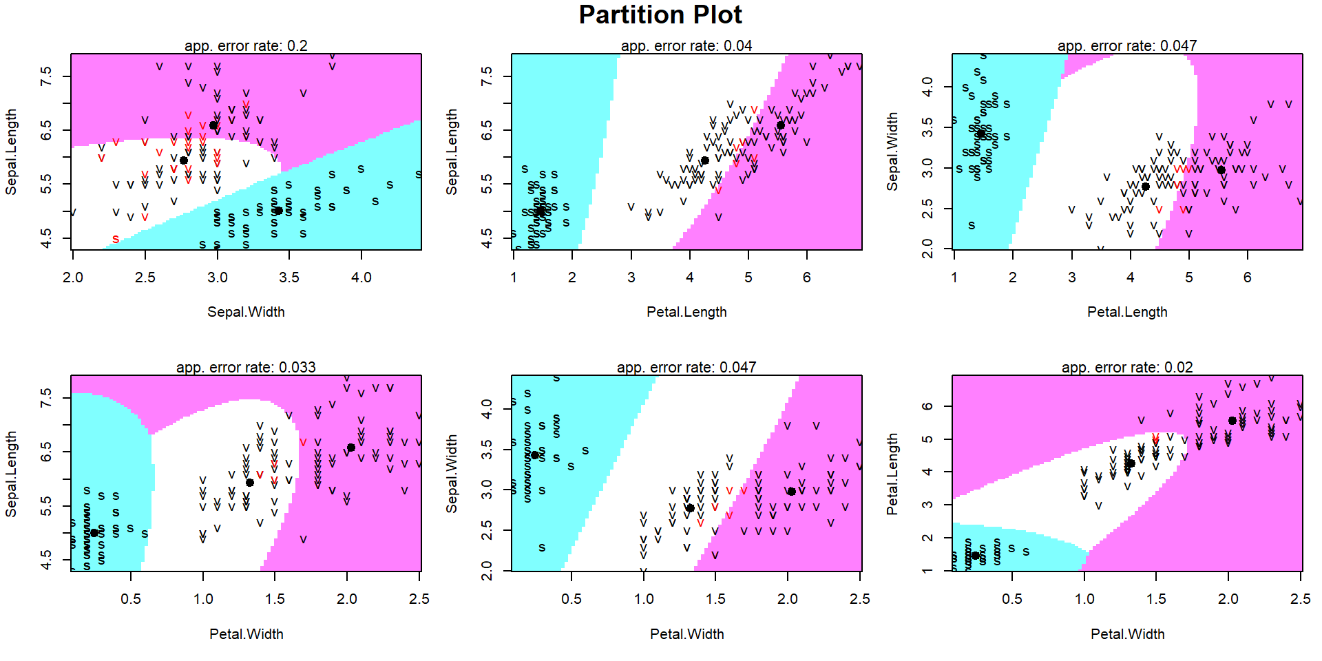
Example of QDA
Example of QDA
            True
Pred         setosa versicolor virginica
  setosa         50          0         0
  versicolor      0         48         1
  virginica       0          2        49
True
Pred setosa versicolor virginica
setosa 50 0 0
versicolor 0 48 1
virginica 0 2 49- The same result for this particular example
Visualize QDA Results
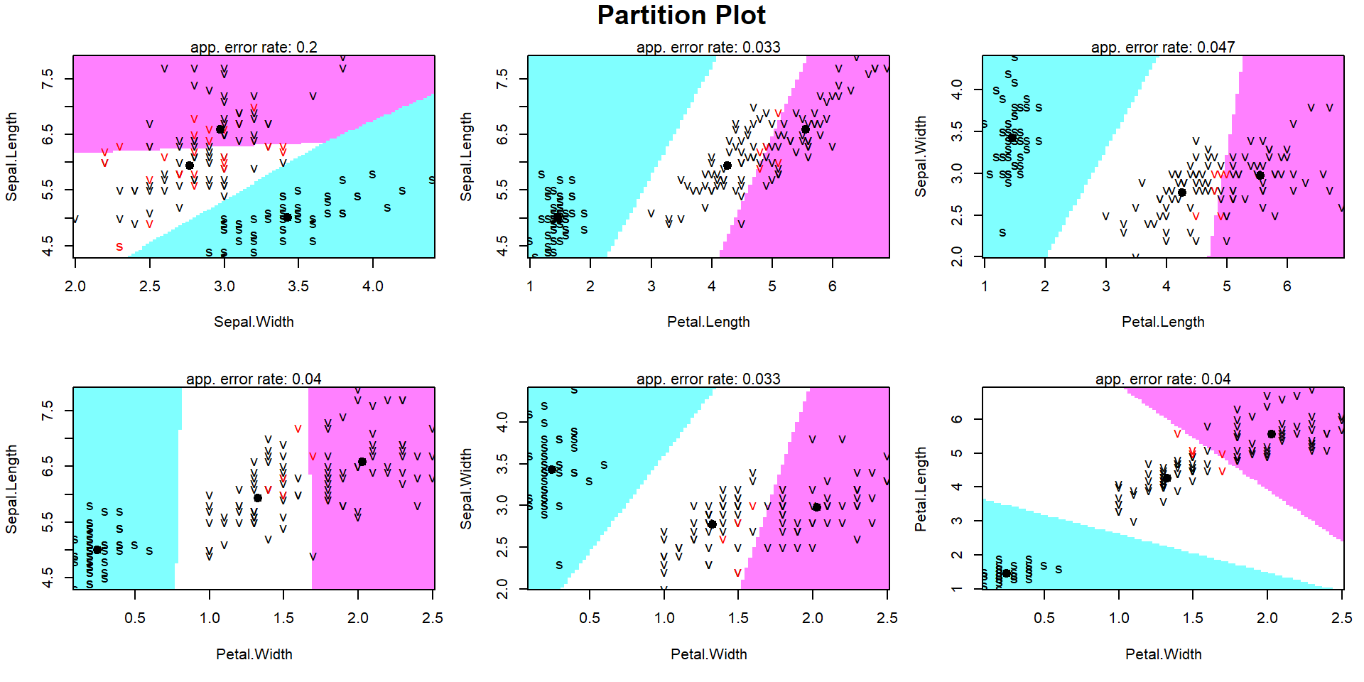
Visualize LDA Results
Decision Theory
Cost and Prior Probabilities
- In practice, different types of errors have different costs
- Prior probabilities are often known but we haven’t discussed how to use them
- Goals:
- When different errors have the same cost, we look for a classification rule that minimizes the probability of misclassification
- When different errors cost differently, we want to find a classification rule that minimizes the total cost
- When different errors have the same cost, we look for a classification rule that minimizes the probability of misclassification
Equal Costs
Minimize Probability of Misclassification
- Notations:
- \(X\): data
- \(Z\): true class. It is binary, i.e., \(Z=1\) or \(Z=0\)
- \(P(Z=1)=\pi\): prior probability, known
- \(\delta(x)\): decision function / classifier
- \(\delta(x)=1\): allocate \(x\) to group 1
- \(\delta(x)=0\): allocate \(x\) to group 0
Risk and Posterior Risk
Risk of a classifier \(\delta\) \[\begin{aligned} R(\delta, z)&=\Pr [\delta(X)\not= Z|Z=z]=\mathbb E_{X|z} [\mathbb I_{\delta(X)\not= Z}|Z=z]\\ &=\left\{ \begin{array}{cc} \Pr[\delta(X)=0|z=1] & \mbox{ if } z=1\\ \Pr[\delta(X)=1|z=0] & \mbox{ if } z=0 \end{array}\right. \end{aligned}\]
The posterior risk of \(\delta\) \[\begin{aligned} PR(\delta(x)) &= \Pr[\delta(x)\not= Z|x]=\mathbb E_{Z|x} [\mathbb I_{\delta(X)\not= Z}|X=x]\\ &=\left\{ \begin{array}{cc} \Pr[Z=0|x] & \mbox{ if } \delta(x)=1\\ \Pr[Z=1|x] & \mbox{ if } \delta(x)=0 \end{array}\right. \end{aligned}\]
Bayes Risk
Bayes risk \(B(\delta)=\Pr [\delta(X)\not= Z]\).
Note that \[B(\delta)=\Pr [\delta(X)\not= Z]=\mathbb E_{XZ} [\mathbb I_{\delta(X)\not= Z}]=E_X[PR(\delta, X)]=E_Z[R(\delta, Z)]\]
Rewrite the Bayes risk \[\begin{aligned} B(\delta) &=\Pr [\delta(X)\not= Z]\\ &=\Pr [\delta(X)=1, Z=0] + \Pr [\delta(X)=0, Z=1]\\ &=\Pr [\delta(X)=1| Z=0]\Pr[Z=0] + \Pr [\delta(X)=0| Z=1] \Pr[Z=1]\\ &=\pi \Pr [\delta(X)=0| Z=1]+ (1-\pi)\Pr [\delta(X)=1| Z=0] \end{aligned}\]
The above expression is baesd on the fact \[B(\delta)=\mathbb E_{XZ} [\mathbb I_{\delta(X)\not= Z}]\]
Bayes Classification Rule
- Want to find \(\delta^*\) that minimizes \(B(\delta)\)
- Claim 1: the \(\delta^*\) that minimizes \(PR(\delta(x))\) also minimizes \(B(\delta)\)
- This is because \(B(\delta)=\mathbb E[PR(\delta(X)]\ge \mathbb E[PR(\delta^*(X)]=B(\delta^*)\)]
- Need to find \(\delta^*\) that minimizes \(PR(\delta(x))\). It can be shown that
\[\delta^*(x)=\left\{ \begin{array}{cc} 1 & \mbox{ if } \frac{\Pr(Z=1|x)}{\Pr(Z=0|x)}>1\\ 0 & \mbox{ if } \frac{\Pr(Z=1|x)}{\Pr(Z=0|x)}<1 \end{array}\right.\]
- Skip next slide if you are not interested in the proof
The Classifier that Minimizes Posterior Risk
- Recall that \[PR(\delta(x)=0)=\Pr(Z=1|x), PR(\delta(x)=1)=\Pr(Z=0|x)\]
- Therefore, we \(\delta^*(x)\) should be 1 if \[\begin{aligned} PR(\delta(x)=0)>PR(\delta(x)=1) &\Leftrightarrow \Pr(Z=1|x)> \Pr(Z=0|x)\\ &\Leftrightarrow \frac{\Pr(Z=1|x)}{\Pr(Z=0|x)}>1 \end{aligned}\]
The Bayes Classificatin Rule
We say \(\delta^*(x)\) is the Bayes classification rule \[\delta^*(x)=\left\{ \begin{array}{cc} 1 & \mbox{ if } \frac{\Pr(Z=1|x)}{\Pr(Z=0|x)}>1\\ 0 & \mbox{ if } \frac{\Pr(Z=1|x)}{\Pr(Z=0|x)}<1 \end{array}\right.\]
Computation \[\begin{aligned} \frac{\Pr(Z=1|x)}{\Pr(Z=0|x)} & \overset{\mbox{Bayes' theorem}} = \frac{\frac{f(x|z=1)\Pr(Z=1)}{f(x)}}{\frac{f(x|z=0)\Pr(Z=0)}{f(x)}}\\ & = \frac{f(x|z=1)}{f(x|z=0)}\frac{\pi}{1-\pi} \end{aligned}\]
A short review of Bayes’ theorem is on next slide. Feel free to skip if you are very familiar with it already
Bayes’ Theorem
- Read this slide if you would like to review Bayes’ theorem
- Let \(A\) and \(B\) be two events.
- Bayes’ theorem says \[\Pr(B|A) = \dfrac{\Pr(A, B)}{\Pr(A)}=\dfrac{\Pr(A|B)\Pr(B)}{\Pr(A)}\] where \(\Pr(A,B)\) means the joint probability that both \(A\) and \(B\) occur. We can use alternative expressions such as \(\Pr(A \text{ and } B)\) and \(\Pr(A \cap B)\).
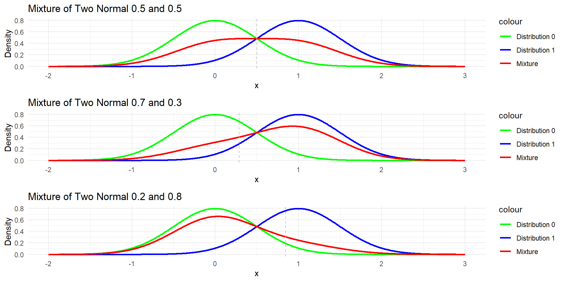
Example 1: Univariate
- Let’s consider a univariate example. Suppose that the population consists for two underlying populations
- Population 1 with \(\pi\) probability and \(N(\mu_1=1, \sigma^2=0.25)\)
- population 0 with \(1-\pi\) probability and \(N(\mu_0=0, \sigma^2=0.25)\)
- Would like to allocate \(x=0.8\)
- According to Bayes classification rule, we need to compute
\[\begin{aligned} \frac{f(x|z=1)\pi}{f(x|z=0)(1-\pi)} &=\frac{f(x|\mu_1=1,\sigma^2)\pi}{f(x|\mu_0=0, \sigma^2)(1-\pi)}\\ &=\frac{\frac{1}{\sigma\sqrt{2\pi}}exp\{-\frac{1}{2\sigma^2}(x-1)^2\}} {\frac{1}{\sigma\sqrt{2\pi}}exp\{-\frac{1}{2\sigma^2}(x-0)^2\}}\frac{\pi}{1-\pi}\\ &= exp\{\frac{1}{2\sigma^2} (2x-1) \}\frac{\pi}{1-\pi} \end{aligned}\]
Example 1: Univariate
The classification boundary is \[\begin{aligned} exp\{\frac{1}{2\sigma^2} (2x-1) \} =(1-\pi)/\pi &\Leftrightarrow \frac{1}{2\sigma^2} (2x-1)=log((1-\pi)/\pi)\\ &\Leftrightarrow x=\sigma^2 log((1-\pi)/\pi)+0.5 \end{aligned}\]
The boundary is linear!
- If \(\pi=0.5\), the boundary is \(x=0.5\), we classify \(x=0.8\) to class 1.
- If \(\pi=0.7\), the boundary is \(x=0.288\), we classify \(x=0.8\) to class 1.
- If \(\pi=0.2\), the bondary is \(x=0.846\), we classify \(x=0.8\) to class 0.
Example 1: Density and Classification Boundary
Example 2: Multivariate
- For a two-class problem, the classification boundary by Bayes’ classification rule is \[\frac{f(x|z=1)\pi}{f(x|z=0)(1-\pi)}=1\\ \Leftrightarrow log(\frac{f(x|z=1)}{f(x|z=0)})=log(\frac{1-\pi}{\pi})\]
Bayes’ Classification under Equal Covariance
Suppose the two underlying distributions are \(N(\boldsymbol\mu_1, \boldsymbol \Sigma)\) and \(N(\boldsymbol\mu_2, \boldsymbol \Sigma)\).
The boundary is \[-\frac{1}{2}(x-\boldsymbol\mu_1)^T \boldsymbol\Sigma^{-1}(x-\boldsymbol\mu_1) + \frac{1}{2}(x-\boldsymbol\mu_1)^T \boldsymbol\Sigma^{-1}(x-\boldsymbol\mu_1)\\ =log(\frac{1-\pi}{\pi})\] which is equivalent to
\[(\boldsymbol\mu_1 -\boldsymbol\mu_2)^T \boldsymbol\Sigma^{-1}x = (\boldsymbol\mu_1 -\boldsymbol\mu_2)^T\boldsymbol\Sigma^{-1}\frac{\boldsymbol\mu_1 + \boldsymbol\mu_2}{2} + log(\frac{1-\pi}{\pi})\]
Bayes’ Classification under Equal Covariance
In practice, we substitute the unknown parameters by their estimates \[(\bar {\mathbf X}_{1.} -\bar {\mathbf X}_{2.})^T\boldsymbol\Sigma^{-1}x = (\bar {\mathbf X}_{1.} -\bar {\mathbf X}_{2.})^T \boldsymbol\Sigma^{-1}\frac{\bar {\mathbf X}_{1.} + \bar {\mathbf X}_{2.}}{2} + log(\frac{1-\pi}{\pi})\]
Recall that in LDA the linear boundary is \[a^Tx=a^T\frac{\bar {\mathbf X}_{1.} + \bar {\mathbf X}_{2.}}{2}\] Therefore, Bayes’ classification is the same as the LDA when \(\pi=1/2\).
Similarly, in a g-class problem, LDA is the same as Bayes classification under the assumptions (1) multivariate normality, (2) equal covariance, and (3) uniform prior probabilities.
Connection with Logistic Regression
- The ratio of posterior risk is \[\frac{\Pr(Z=1|x)}{{\Pr(Z=0|x)}}\]
- It is also called the odds ratio. A logistic regression models the log-odds as a linear function of the covariates.
- The LDA under the Bayes rule computes the ratio of the posterior risk.
Connection with Logistic Regression
- In both approaches, the decision function is a linear function of the covariates.
- They also give similar results.
- The two approaches were derived from different models with different assumptions.
- Logistic regression models the behavior of a binary response variable given covariates.
- LDA models the multivariate behavior of covariates given the class labels.
- If MVN is not satisfied, LDA is not a good approximation to the posterior risk. In this situation, logistic regression is a better choice.
Example 3: Univariate, Unequal Variance
- Again, consider a univariate example. This time we relax the assumption of equal variance
- Suppose that the population consists for two underlying populations
- Population 1 with \(\pi\) probability and \(N(\mu_1=1, \sigma_1^2=0.25)\)
- population 0 with \(1-\pi\) probability and \(N(\mu_0=0, \sigma_2^2=1)\)
- Would like to allocate \(x=0.8\)
Example 3: Univariate, Unequal Variance
- According to Bayes classification rule, we need to compute \[\begin{aligned} \frac{f(x|z=1)\pi}{f(x|z=0)(1-\pi)} &=\frac{f(x|\mu_1=1,\sigma_1^2)\pi}{f(x|\mu_0=0, \sigma_0^2)(1-\pi)}\\ &=\frac{\frac{1}{\sigma_1\sqrt{2\pi}}exp\{-\frac{1}{2\sigma_1^2}(x-1)^2\}} {\frac{1}{\sigma_0\sqrt{2\pi}}exp\{-\frac{1}{2\sigma_0^2}(x-0)^2\}}\frac{\pi}{1-\pi}\\ &= exp\{(\frac{1}{2\sigma_0^2}-\frac{1}{2\sigma_1^2})x^2 + \frac{x}{\sigma_1^2}-\frac{1}{2\sigma_1^2}\} \frac{\pi}{1-\pi}\frac{\sigma_0}{\sigma_1} \end{aligned}\]
Example 3: Univariate, Unequal Variance
The classification boundary is \[(\frac{1}{2\sigma_0^2}-\frac{1}{2\sigma_1^2})x^2 + \frac{x}{\sigma_1^2}-\frac{1}{2\sigma_1^2}=log[ \frac{1-\pi}{\pi}\frac{\sigma_1}{\sigma_0}] \]
It is quadratic!
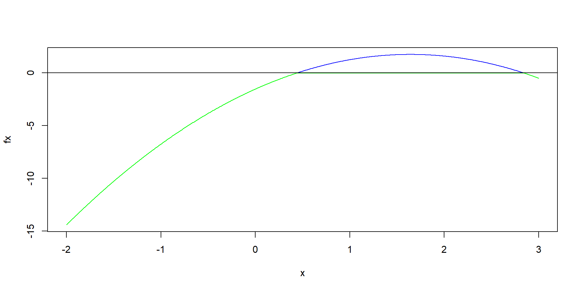
Example 3: Univariate, Unequal Variance
Code
mean1 <- 1
var1 <- 0.25
mean0 <- 0
var0 <- 0.64
weight1 <- 0.5
weight0 <- 1 - weight1

# doesn't seem to be correct
x <- seq(-2, 3, length.out = 1000)
fx=(1/var0 - 1/var1)/2*x^2 + x/var1 - 1/2/var1 - log(weight0*sqrt(var1)/weight1/sqrt(var0))
plot(x, fx, type="n")
lines(x[fx>0], fx[fx>0], col="blue")
lines(x[fx<0], fx[fx<0], col="green")
abline(h=0)
Example 3: Univariate, Unequal Variance
Unequal Costs
Risk and Cost
- Different types of misclassifications might cost differently
- Let \(L(\delta(x), z)\) denote the cost function
- Let \(C(1|0)=L(1, 0)\), the cost of misclassifying 0 to 1
- Let \(C(0|1)=L(0, 1)\), the cost of misclassifying 1 to 0
- The Risk and Bayes risk need to be revised accordingly
Risk and Posterior Risk
Risk of a classifier \(\delta\) \[R(\delta, z)=\mathbb E_{X|Z=z} [L(\delta(X), z)]=\left\{ \begin{array}{cc} C(0|1)\Pr[\delta(X)=0|z=1] & \mbox{ if } z=1\\ C(1|0)\Pr[\delta(X)=1|z=0] & \mbox{ if } z=0 \end{array}\right.\]
The posterior risk of \(\delta\) \[\begin{aligned} PR(\delta(x)) &= \mathbb E_{Z|x}[L(\delta(x), Z)]\\ &=\left\{ \begin{array}{cc} C(1|0)\Pr[Z=0|x] & \mbox{ if } \delta(x)=1\\ C(0|1)\Pr[Z=1|x] & \mbox{ if } \delta(x)=0 \end{array}\right. \end{aligned}\]
Bayes Risk
- Bayes risk \[B(\delta)=\mathbb E_{XZ} [L(\delta(X), Z)]\]
- Rewrite the Bayes risk
\[\begin{aligned} B(\delta) &=\mathbb E_{XZ} [L(\delta(X), Z)]\\ &=L(\delta(X)=1, Z=0)\Pr[\delta(X)=1, Z=0] + L(\delta(X)=0, Z=1)[\delta(X)=0, Z=1]\\ &=C(1|0)\Pr [\delta(X)=1, Z=0] + C(0|1)\Pr [\delta(X)=0, Z=1]\\ &=C(1|0)\Pr [\delta(X)=1| Z=0]\Pr[Z=0] + C(0|1)\Pr [\delta(X)=0| Z=1] \Pr[Z=1]\\ &=C(0|1)\pi \Pr [\delta(X)=0| Z=1]+ (1-\pi)C(1|0)\Pr [\delta(X)=1| Z=0] \end{aligned}\]
Bayes Classification Rule with Unequal Costs
- Use a derivation similar to the equal cost situation, we can show that the Bayes classification rule is
\[\begin{aligned} &PR(\delta(x)=0)>PR(\delta(x)=1) \\ &\Leftrightarrow C(0|1)\Pr(Z=1|x)> C(1|0)\Pr(Z=0|x)\\ &\Leftrightarrow \frac{\Pr(Z=1|x)}{\Pr(Z=0|x)}>\frac{C(1|0)}{C(0|1)}\\ &\Leftrightarrow \frac{f(x|z=1)}{f(x|z=0)}>\frac{C(1|0)}{C(0|1)}\frac{1-\pi}{\pi} \end{aligned}\]
Other Related Topics
- There are numerous issues/methods / models
- Training error vs testing error
- Model / variable selection / shrinkage
- Classification tree. Random forest
- Support vector machine
- Neural network and deep neural network